Section 6.2: One-Way ANOVA Assumptions, Interpretation, and Write Up

One-Way ANOVA Assumptions

There are a number of assumptions that need to be met before performing a Between Groups ANOVA:

1. The dependent variable (the variable of interest) needs to be a continuous scale (i.e., the data needs to be at either an interval or ratio measurement).
2. The independent variable needs to have two independent groups with two levels. When testing three or more independent, categorical groups it is best to use a one-way ANOVA, The test could be used to test the difference between just two groups, however, an independent samples t-test would be more appropriate.
3. The data should have independence of observations (i.e., there shouldn’t be the same participants who are in both groups.)
4. The dependent variable should be normally or near-to-normally distributed for each group. It is worth noting that while the t-test is robust for minor violations in normality, if your data is very non-normal, it would be worth using a non-parametric test or bootstrapping (see later chapters).
5. There should be no spurious outliers.
6. The data must have homogeneity of variances. This assumption can be tested using Levene’s test for homogeneity of variances in the statistics package. which is shown in the output included in the next chapter.

Sample Size

A consideration for ANOVA is homogeneity. Homogeneity, in this context, just means that all of the groups’ distribution and errors differ in approximately the same way, regardless of the mean for each group. The more incompatible or unequal the group sizes are in a simple one-way between-subjects ANOVA, the more important the assumption of homogeneity is. Unequal group sizes in factorial designs can create ambiguity in results. You can test for homogeneity in PSPP and SPSS. In this class, a significant result indicates that homogeneity has been violated.

Equal cell Sizes

It is preferable to have similar or the same number of observations in each group. This provides a stronger model that tends not to violate any of the assumptions. Having unequal groups can lead to violations in normality or homogeneity of variance.

One-Way ANOVA Interpretation

Below you click to see the output for the ANOVA test of the Research Question, we have included the research example and hypothesis we will be working through is: Is there a difference in reported levels of mental distress for full-time, part-time, and casual employees?

Main Effects

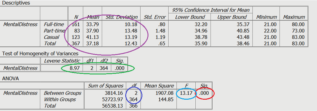
As can be seen in the circled section in red on Slide 3, the main effect was significant. By looking at the purple circle, we can see the means for each group. In the light blue circle is the test statistic, which in this case is the F value. Finally, in the dark blue circle, we can see both values for the degrees of freedom.

Posthoc Tests

In order to run posthoc tests, we need to enter some syntax. This will be covered in the slides for this section, so please do go and have a look at the syntax that has been used. The information has also been included on Slide 4.

Posthoc Test Results

These are the results. There are a number of different tests that can be used in posthoc differences tests, to control for type 1 or type 2 errors, however, for this example none have been used.

Results

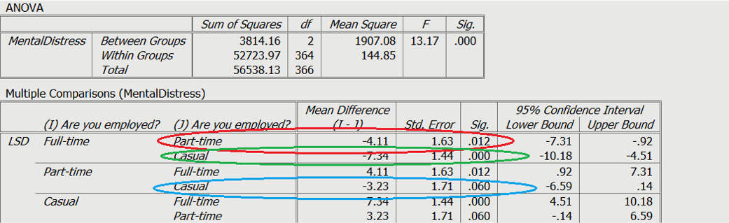
As can be seen in the red and green circles on Slide 6, both part-time and casual workers reported higher mental distress than full-time workers. This can be cross-referenced with the means on the results slide. As be seen in blue, there was not a significant difference between casual and part-time workers.

One-Way ANOVA Write Up

The following text represents how you may write up a One Way ANOVA:

A one-way ANOVA was conducted to determine if levels of mental distress were different across employment status. Participants were classified into three groups: Full-time (n = 161), Part-time (n = 83), Casual (n = 123). There was a statistically significant difference between groups as determined by one-way ANOVA (F(2,364) = 13.17, p < .001). Post-hoc tests revealed that mental distress was significantly higher in participants who were part-time and casually employed, when compare to full-time (Mdiff  = 4.11, p = .012, and Mdiff  = 7.34, p < .001, respectively). Additionally, no difference was found between participants who were employed part-time and casually (Mdiff  =3.23, p = .06).