Section 5.3: Multiple Regression Explanation, Assumptions, Interpretation, and Write Up

Multiple Regression is a step beyond simple regression. The main difference between simple and multiple regression is that multiple regression includes two or more independent variables – sometimes called predictor variables – in the model, rather than just one.

As such, the purpose of multiple regression is to determine the utility of a set of predictor variables for predicting an outcome, which is generally some important event or behaviour. This outcome can be designated as the outcome variable, the dependent variable, or the criterion variable. For example, you might hypothesise that the need to belong will predict motivations for Facebook use and that self-esteem and meaningful existence will uniquely predict motivations for Facebook use.

Before beginning your analysis, you should consider the following points:

• Regression analyses reveal relationships among variables (relationship between the criterion variable and the linear combination of a set of predictor variables) but do not imply a causal relationship.
• A regression solution – or set of predictor variables – is sensitive to combinations of variables. Whether a predictor is important in a solution depends on the other predictors in the set. If the predictor of interest is the only one that assesses some important facet of the outcome, it will appear important. If a predictor is only one of several predictors that assess the same important facet of the outcome, it will appear less important.  For a good set of predictor variables – the smallest set of uncorrelated variables is best.

In these Venn Diagrams, you can see why it is best for the predictors to be strongly correlated with the dependent variable but uncorrelated with the other Independent Variables. This reduces the amount of shared variance between the independent variables.  The illustration in Slide 2 shows logical relationships between predictors, for two different possible regression models in separate Venn diagrams. On the left, you can see three partially correlated independent variables on a single dependent variable. The three partially correlated independent variables are physical health, mental health, and spiritual health and the dependent variable is life satisfaction. On the right, you have three highly correlated independent variables (e.g., BMI, blood pressure, heart rate) on the dependent variable of life satisfaction. The model on the left would have some use in discovering the associations between those variables, however, the model on the right would not be useful, as all three of the independent variables are basically measuring the same thing and are mostly accounting for the same variability in the dependent variable.

There are two main types of regression with multiple independent variables:

• Standard or Single Step: Where all predictors enter the regression together.
• Sequential or Hierarchical:  Where all predictors are entered in blocks. Each block represents one step.

We will now be exploring the single step multiple regression:

All predictors enter the regression equation at once. Each predictor is treated as if it had been analysed in the regression model after all other predictors had been analysed. These predictors are evaluated by the shared variance (i.e., level of prediction) shared between the dependant variable and the individual predictor variable.

Multiple Regression Assumptions

There are a number of assumptions that should be assessed before performing a multiple regression analysis:

1. The dependant variable (the variable of interest) needs to be using a continuous scale.
2. There are two or more independent variables. These can be measured using either continuous or categorical means.
3. The three or more variables of interest should have a linear relationship, which you can check by using a scatterplot.
4. The data should have homoscedasticity. In other words, the line of best fit is not dissimilar as the data points move across the line in a positive or negative direction. Homoscedasticity can be checked by producing standardised residual plots against the unstandardized predicted values.
5. The data should not have two or more independent variables that are highly correlated. This is called multicollinearity which can be checked using Variance-inflation-factor or VIF values. High VIF indicates that the associated independent variable is highly collinear with the other variables in the model.
6. There should be no spurious outliers.
7. The residuals (errors) should be approximately normally distributed. This can be checked by a histogram (with a superimposed normal curve) and by plotting the of the standardised residuals using either a P-P Plot, or a Normal Q-Q Plot .

Multiple Regression Interpretation

For our example research question, we will be looking at the combined effect of three predictor variables – perceived life stress, location, and age – on the outcome variable of physical health? 

Slide 1 contains the standard regression analysis output.

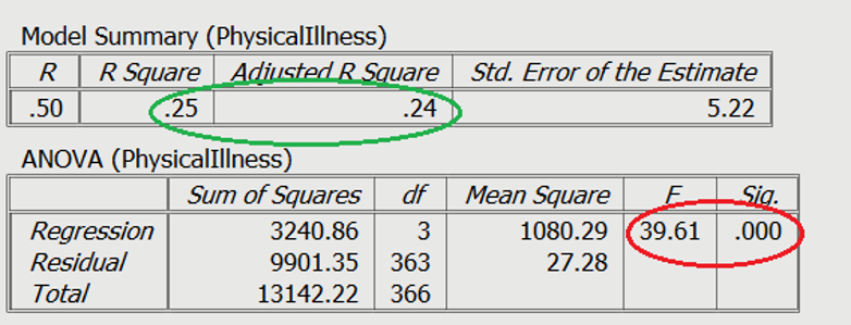
On Slide 2 you can see in the red circle, the test statistics are significant.  The F-statistic examines the overall significance of the model, and shows if your predictors as a group provide a better fit to the data than no predictor variables, which they do in this example.

The R² values are shown in the green circle. The R² value shows the total amount of variance accounted for in the criterion by the predictors, and the adjusted R² is the estimated value of  R² in the population. 

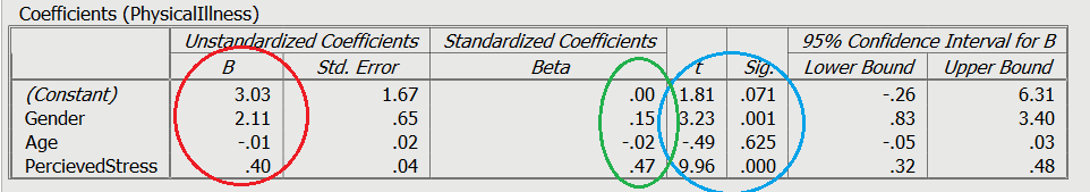
Moving on to the individual variable effects on Slide 3, you can see the significance of the contribution of individual predictors in light blue. The unstandardized slope or the B value is shown in red, which represents the change caused by the variable (e.g., increasing  1 unit of perceived stress will raise physical illness by .40). Finally, you can see the standardised slope value in green, which are also known as beta values. These values are standardised ranging from +/-0 to 1, similar to an r value.  

We should also briefly discuss dummy variables:

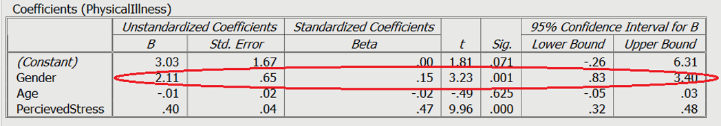
A dummy variable is a variable that is used to represent categorical information relating to the participants in a study. This could include gender, location, race, age groups, and you get the idea.  Dummy variables are most often represented as dichotomous variables (they only have two values). When performing a regression, it is easier for interpretation if the values for the dummy variable is set to 0 or 1. 1 usually resents when a characteristic is present. For example, a question asking the participants “Do you have a drivers license” with a forced choice response of yes or no.

In this example on Slide 3 and circled in red, the variable is gender with male = 0, and female = 1. A positive Beta (B) means an association with 1, whereas a negative beta means an association with 0. In this case, being female was associated with greater levels of physical illness.

Multiple Regression Write Up

Here is an example of how to write up the results of a standard multiple regression analysis:

In order to test the research question, a multiple regression was conducted, with age, gender (0 = male, 1 = female), and perceived life stress as the predictors, with levels of physical illness as the dependent variable. Overall, the results showed the utility of the predictive model was significant, F(3,363) = 39.61, R2 = .25, p< .001. All of the predictors explain a large amount of the variance between the variables (25%).  The results showed that perceived stress and gender of participants were significant positive predictors of physical illness (β=.47, t= 9.96, p< .001, and β=.15, t= 3.23, p= .001, respectively). The results showed that age (β=-.02, t= -0.49 p= .63) was not a significant predictor of perceived stress.