Section 3.4: Paired T-test Assumptions, Interpretation, and Write Up
Learning Objectives
At the end of this chapter you should be able to answer the following questions:
- How does the Paired t-test differ from the Independent t-test?
- What assumptions that need to be met before performing a Paired-samples t-test?
- What elements or individual statistics should be reported when writing up a Paired T-test?
The Paired t-test is also known as the Paired Samples t-test or the Dependent t-test.
Paired T-test Assumptions
Just like in the Independent t-test from our previous chapter, there are a number of assumptions that need to be met before performing a Paired-samples t-test:
- The dependent variable (the variable of interest) needs a continuous scale (i.e., the data needs to be at either an interval or ratio measurement). An example of this variable could be weight or level of anxiety.
- The independent variable must have two groups that are related or have “matched pairs”. Matched pairs, as mentioned above, mean that the same participants are present in both groups. More specifically, we are measuring the same persons twice.
- There should be no spurious outliers across either of the groups being used in the test.
- There should be an approximate normal distribution of differences across the two related groups.
Paired T-test Interpretation
A Paired t-tests examines the within-group differences of a single group. So the same subjects are the respondents for both pairs of measurements, and this indicates that you have related groups of scores.
This means that the “related groups” or “matched pairs” are the same participants who have been measured in each of the two groups. Specifically this means the two groups both contain the same people, who are producing the same scores or measurements in both groups. Unlike the independent samples t-test, researchers can measure the same participants in each level of the independent variable because the measurement or scoring for each participant will be taken at two distinct time points.
In the worked example for this test, we will be looking at the levels of perceived social support a group of Australians reported before engaging with a social skills building program and after completing the program.
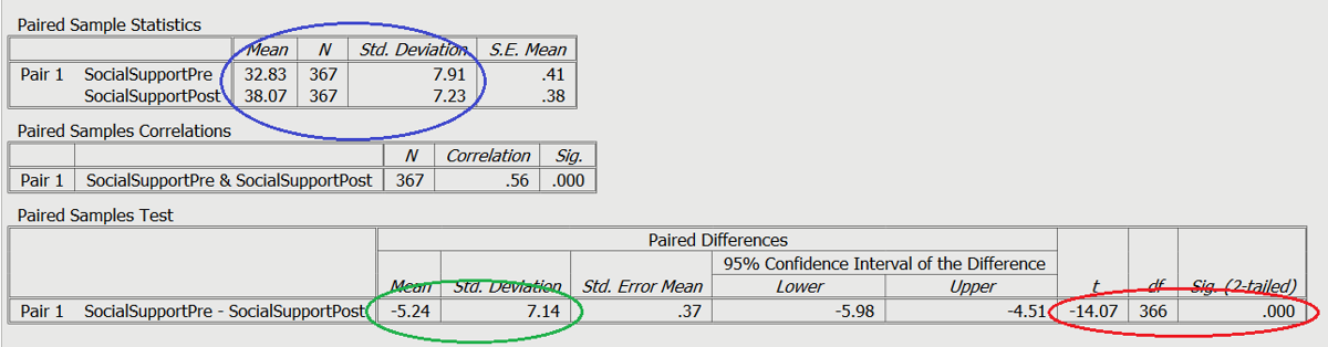
Red: Test statistics
Green: Differences in means for effect size
Blue: Means and standard deviation
This example shows perceived social support as an outcome variable. This outcome is expected to change after the intervention of a social skills building program.
The output shows levels of perceived social support across two groups of scores: Scores from a group of Australians reported before engaging with a social skills building program, and scores the same people reported after completing the program.
As you can see, the t-test was significant as circled in red, showing a change from the scores before completing the social skills program, and after. By looking at the means as circled in blue you can tell that the mean level of perceived social support was higher following the completion of the program. To calculate the effect size, you divide the mean difference by the standard deviation of the difference as circled in green.
Paired T-test Write Up
When you are writing your report, you will need to include the Means and SD for each group, along with the t test statistic (t), its p value, and its effect size d.
A Write-Up for a Paired T-test should look like this:
A paired samples t-test showed that the participant’s level of perceived social support increased from pre-program (M = 32.83, SD = 7.91) to post-program (M = 38.07, SD = 7.23; t = -14.07, p < .001, d = -.73).
