Section 5.4: Hierarchical Regression Explanation, Assumptions, Interpretation, and Write Up

Hierarchical Regression Explanation and Assumptions

Hierarchical regression is a type of regression model in which the predictors are entered in blocks. Each block represents one step (or model). The order (or which predictor goes into which block) to enter predictors into the model is decided by the researcher, but should always be based on theory.

The first block entered into a hierarchical regression can include “control variables,” which are variables that we want to hold constant. In a sense, researchers want to account for the variability of the control variables by removing it before analysing the relationship between the predictors and the outcome.

The example research question is “what is the effect of perceived stress on physical illness, after controlling for age and gender?”.  To answer this research question, we will need two blocks. One with age and gender, then the next block including perceived stress.

It is important to note that the assumptions for hierarchical regression are the same as those covered for simple or basic multiple regression. You may wish to go back to the section on multiple regression assumptions if you can’t remember the assumptions or want to check them out before progressing through the chapter.

Hierarchical Regression Interpretation

For this test, the statistical program used was Jamovi, which is freely available to use. The first two slides show the steps to get produce the results. The third slide shows the output with any highlighting. You might want to think about what you have already learned, to see if you can work out the important elements of this output.

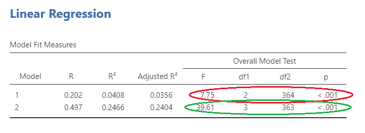
Slide 2 shows the overall model statistics. The first model, with only age and gender, can be seen circled in red. This model is obviously significant. The second model (circled in green) includes age, gender, and perceived stress. As you can see, the F statistic is larger for the second model. However, does this mean it is significantly larger?

To answer this question, we will need to look at the model change statistics on Slide 3. The R value for model 1 can be seen here circled in red as .202. This model explains approximately 4% of the variance in physical illness. The R value for model 2 is circled in green, and explains a more sizeable part of the variance, about 25%.

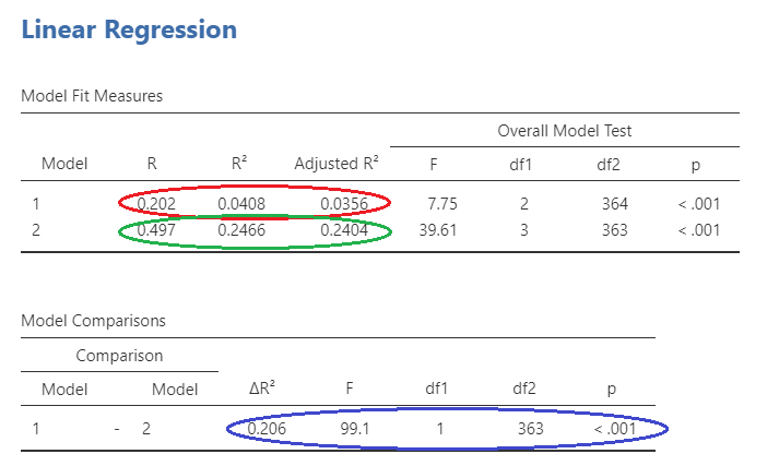
The significance of the change in the model can be seen in blue on Slide 3. The information you are looking at is the R squared change, the F statistic change, and the statistical significance of this change.

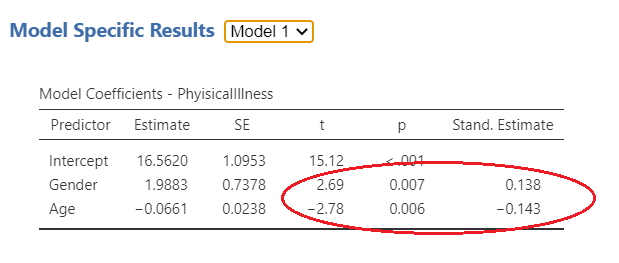
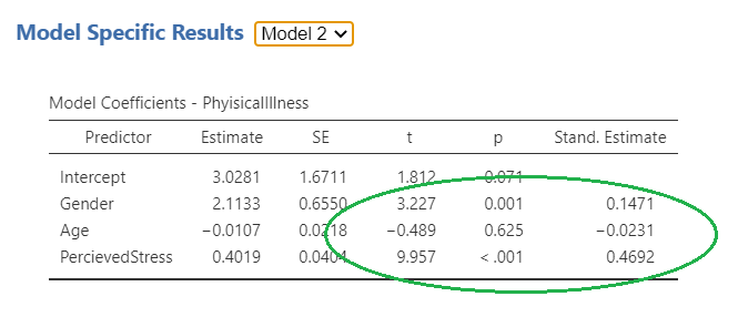
On Slide 4, you can examine the role of each individual independent variable on the dependant variable. For model one, as circled in red, age and gender are both significantly associated with physical illness. In this case, age is negatively associated (i.e. the younger you are, the more likely you are to be healthy), and gender is positively associated (in this case being female is more likely to result in more physical illness).  For model 2, gender is still positively associated and now perceived stress is also positively associated. However, age is no longer significantly associated with physical illness following the introduction of perceived stress. Possibly this is because older persons are experiencing less life stress than younger persons.

Hierarchical Regression Write Up

An example write up of a hierarchal regression analysis is seen below:

In order to test the predictions, a hierarchical multiple regression was conducted, with two blocks of variables. The first block included age and gender (0 = male, 1 = female) as the predictors, with difficulties in physical illness as the dependant variable. In block two, levels of perceived stress was also included as the predictor variable, with difficulties in perceived stress as the dependant variable.

Overall, the results showed that the first model was significant F(2,364) = 7.75, p= .001, R2=.04. Both age and gender were significantly associated with perceived life stress (b=-0.14, t= -2.78, p= .006, and b=.14, t= 2.70, p= .007, respectively). The second model (F(3,363) = 39.61, p< .001, R2=.25), which included physical illness (b=0.47, t= 9.96, p< .001) showed significant improvement from the first model ∆F(1,363) = 99.13, p< .001, ∆R2=.21,  , Overall, when age and location of participants were included in the model, the variables explained 8.6% of the variance, with the final model, including physical illness accounted for 24.7% of the variance, with model one and two representing a small, and large effect size, respectively.