Section 6.3 Repeated Measures ANOVA Assumptions, Interpretation, and Write Up

Let’s look now at a repeated measures ANOVA. A repeated measures ANOVA is used to compare three or more group means when the participants are the same in each group. Usually, this would occur when a participant is repeated tested, particularly if you are evaluating an intervention. For example, you could use a repeated measures ANOVA to better understand whether there is a difference in anxiety levels after a group therapy program. You could measure anxiety levels at three time points, such as at the start of the program, one month after the program is completed, and then six months after the program is completed.

Repeated Measures ANOVA Assumptions

For a Repeated Measures ANOVA there are two or more independent variables (factors) that can be denoted by the levels of each Independent Variable (IV).

For example, in a design with 2 IVs, the ANOVA is described as A X B ANOVA

(A = Number of levels of IV1; B = Numbers of levels of IV2)

Meanings of the levels of factors can change when researchers shift between between-subjects designs and within-subjects designs.

For between-subjects design, levels can be thought of as different groups of the factor.

For within-subjects design, levels can be thought of as different conditions of the factor.

There are also several assumptions that go with Repeated Measures ANOVA:

1. The dependent variable (the variable of interest) needs a continuous scale (i.e., the data needs to be at either an interval or ratio measurement).
2. The “within-groups” variable must have two or more groups that are related or have “matched pairs”. As in the Paired-samples T-test, matched pairs mean that the same participants are present in both groups (i.e. measuring the same persons twice).
3. There should be no spurious outliers.
4. The dependent variable should be normally or near-to-normally distributed for each group. It is worth noting that the t-test is robust for minor violations in normality, however, if your data is very non-normal, it would be worth using a non-parametric test or bootstrapping (see later chapters).
5. The data must have what is known as “sphericity”. This means that amount of variable across the differences for all of the groups (both within and between) must be equal or near-to-equal the variances of the differences between all combinations of related groups must be equal. This can be tested using statistical software.

Repeated Measures ANOVA Interpretation

In our example below, the researchers are interested in the effects of more than 1 IV on a DV, which in this case are the effects of a social support program and gender on perceived levels of life satisfaction.

In the scenario, there are 2 factors or IVs:

Life satisfaction (pre- and post-program: 2 levels) X gender (male and female: 2 levels)

For this test, the statistical program used was Jamovi, which is freely available to use. The first two slides show the steps to get produce the results. The third slide shows the output with any highlighting.

Hypothesis

Often when using an ANOVA repeated measures design, three or more different hypotheses are testable. A main effect of factor 1, a main effect of factor 2, and an interaction effect of both factor 1 and factor 2. As you can see in the figure, there is a 3-way design to this ANOVA = A X B X C

Interaction

Answers the question similar to “moderation effect” in regression

Determines whether differences that can be attributed to a factor are consistent at all levels of the other factor/s or differences that can be attributed to a factor depending on the level of the other factor.

Run the analysis

In this example, we are interested in the effects of more than 1 IV on the DV. In this case, we want to know the effects of a social support program and gender on perceived levels of life satisfaction. We want to know if the program works in improving perceptions of life satisfaction (Factor 2), and if gender can play a role in levels of life satisfaction (Factor 2). Finally, we want to know if both males and females improve at the same rate in the intervention.

In the scenario, there are 2 factors or IVs

Program (pre- and post-program: 2 levels) X gender (male and female: 2 levels)

Effects to test in ANOVA :

• • Main program effect (Time)
  • Main gender effect (Gender)
  • Interaction effect of time and gender

Jamovi Interface

As you can see, there is a number of things to enter into Jamovi, which we will cover in the slides.

Homogeneity

In this case, as we are only texting two groups, and two time points, Homogeneity isn’t a major consideration in the overall analysis. However, as you can see in red, you do want these values to be greater than .05 when testing multiple groups/timepoints.

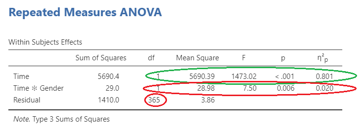
Within groups

The within-groups results can be seen here. In green is the main effect for time, which is our primary within groups variable. The results are significant, which shows a change from pre- to post-scores. The large red circle shows the interaction of gender and time, which is of interest as well. As this interaction is significant, this shows that when moving from pre- to post-intervention, male and female participants scores’ show a different rate of change. The small red circle is the overall degrees of freedom for the model, which you will need when reporting the results.

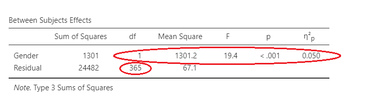
Between groups

As you can see in the large red circle, the results of the between-groups analysis shows that there is a difference between males and females.

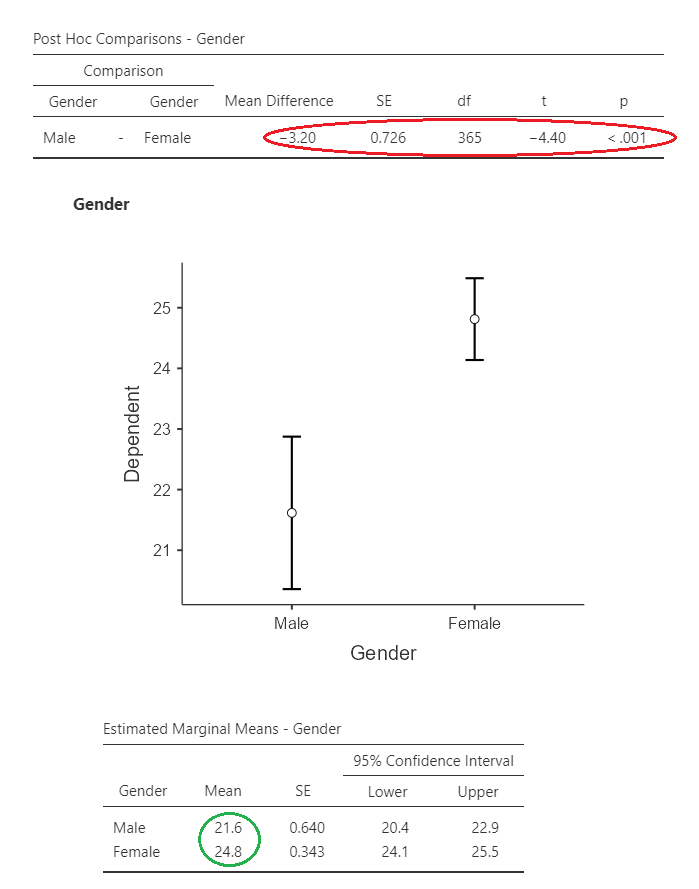
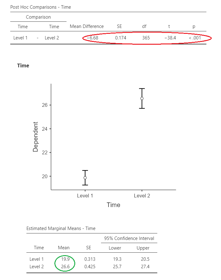
Main effects

The results of the main effects can be seen here. In the green circles are the means for the groups/time points, and in the red is the actual comparison tests. As we can see here, there was an improvement in scores from pre- to post-intervention, and females tended to score more highly.

Interactions

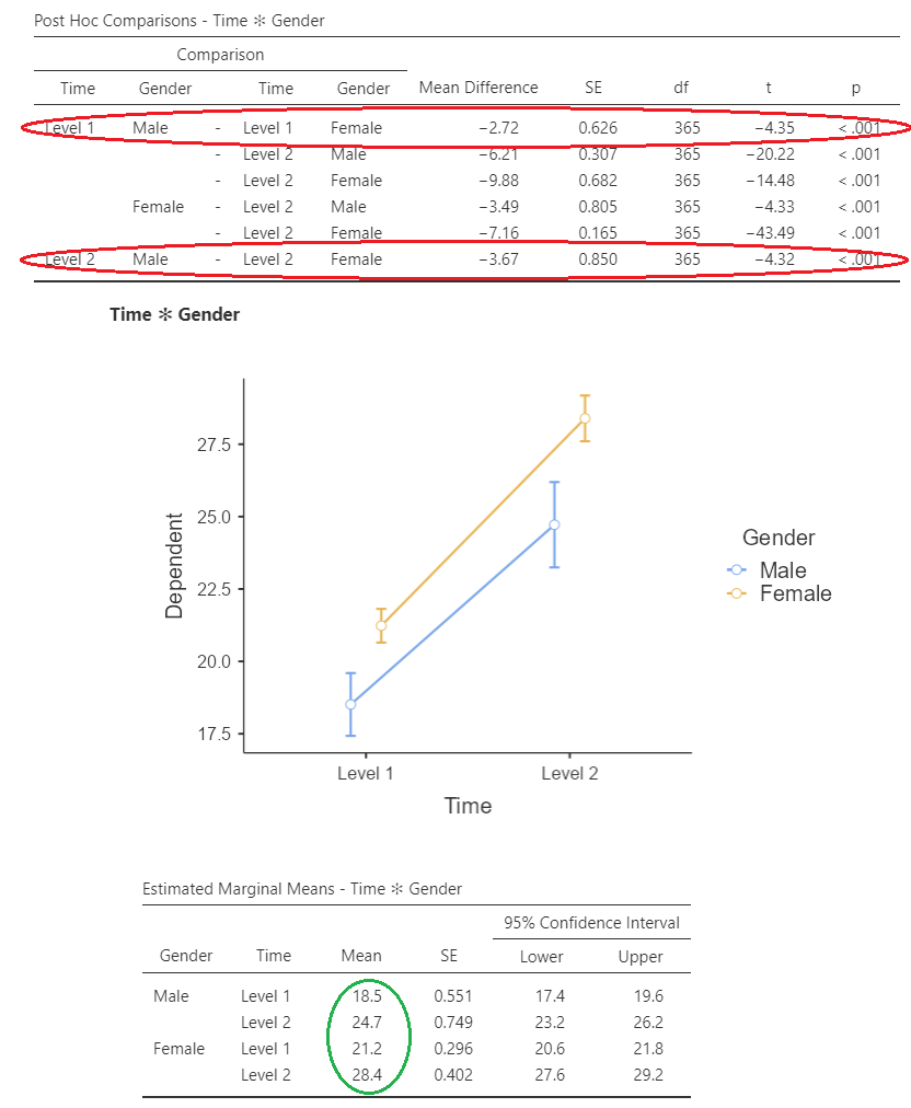
In this case, we have used follow-up post hoc t-tests to test the difference across gender at each timepoint. This is to further examine the interaction of gender and time. The means for each group at each timepoint can be seen in green, and the results of the posthoc are in red. In this case, it is apparent from the results, that while both males and females improved pre to post-intervention, female participants started with greater life satisfaction, and saw greater improvement following the intervention than males.

Repeated Measures ANOVA Write Up

The following presents a write up for a Repeated Measures ANOVA:

The analysis showed both a significant main effect for time, F(1,365) = 1473.02, p < .001, np2 = 0.80, and gender, F(1,365) = 19.40, p < .001, np2 = 0.05, as well as a significant interaction of time and gender F(1,365) = 7.50, p = .006, np2 = 0.02. Two follow up independent samples t-tests were conducted comparing life satisfaction for male and female participants at time 1 and time 2; t(365) = -4.35, p < .001, d = 0.25, and t(365) = 4.32, p < .001, d = 0.27, respectively. The results showed that female participants reported higher scores than males at both pre- and post-intervention. (Graphs should be included when reporting these results.)