Section 5.2: Simple Regression Assumptions, Interpretation, and Write Up

Like in our previous chapters, it is important to understand that simple regression also has assumptions. In this case, Simple Regression Assumptions include:

1. The two variables (the variables of interest) need to be using a continuous scale.
2. The two variables of interest should have a linear relationship, which you can check with a scatterplot.
3. There should be no spurious outliers.
4. The variables should be normally or near-to-normally distributed.

Simple Regression Interpretation

The first slide provides you with an example output in which physical illness is regressed on mental distress scores. In other words, we are using mental distress to predict your physical illness score.

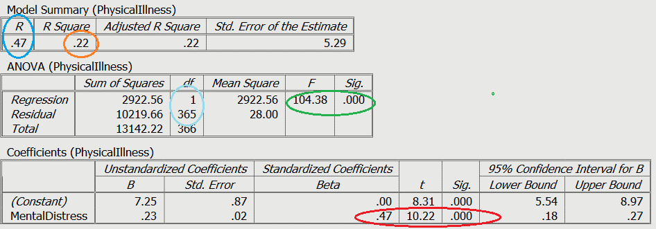
Green: Model statistics

Light Blue: Degrees of Freedom

Blue: R value

Orange: R² value

Red: Variable test statistcs

If you go to the second slide, we have circled certain important elements of the statistical output. For example, you can see the statistics for the overall model, that is, the F statistic and the overall significance of the model which have been circled in green. The degrees of freedom (df) have been circled in light blue (see the ANOVA (Physical Illness) box). Although these statistics are more important in multiple or hierarchical regression, they are useful here because they provide you with an indication of the significance of the overall model. 

The next thing to examine is the significance of the individual predictor variable (circled in red), with the standardised b value (known as beta), the t value, and the significance shown.

Don’t forget to look at the R Squared value (circled in orange), which can be interpreted as a percentage of variance explained in the outcome by the predictor. In this example, mental distress accounts for 22% of the shared variance with physical illness.

Finally, the r value (circled in a darker blue) which is the Pearson correlation coefficient, represents the standardised line of best fit for the model.

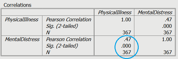
As you can see the r value, shows the same value as the correlation between the two variables, which we discussed in Chapter Four. This is expected in simple regression, but the values for predictors in regression models will change as we include more predictor variables to make a more complex model.  

Simple Regression Write Up

Here is an example of how you can write up the results of a simple regression analysis:

In order to test the research question, a simple regression was conducted, with mental distress as the predictor, and levels of physical illness as the dependent variable. Overall, the results showed that the utility of the predictive model was significant, F(1,365) = 104.38, R2 = .22, p< .001. Mental distress explained a large amount of the variance between the variables (22%).  The results showed that mental distress was a significant positive predictor of physical illness (β=.47, t= 10.22, p< .001).