Section 3.3: Independent T-test Assumptions, Interpretation, and Write Up
Learning Objectives
At the end of this chapter you should be able to answer the following questions:
- Is the Independent T-test a Between Groups or Within Groups test?
- How many assumptions underpin the Independent Samples T-test?
- What is the first test to examine within the Independent Groups T-test output?
- What is the second test to examine within the Independent Groups T-test output?
- What elements or individual statistics should be reported when writing up an Independent T-test?
An Independent T-test or Independent Samples T-test is an important test for Between Groups differences.
Here we will discuss the underlying assumptions of the Independent t-test and explain how to interpret the results of the t-test. There are a number of assumptions that need to be met before performing an Independent t-test:
- The dependent variable (the variable of interest) needs a continuous scale (i.e., the data needs to be at either an interval or ratio measurement). An example of a continuous dependent variable might be the weight of an athlete. Their weight could be anywhere between 50 and 70 kilograms.
- The independent variable needs to have two independent groups with two levels. An example of this independent variable could be regional vs metropolitan Australians.
- The data should have independence of observations. More specifically, there shouldn’t be the same participants in both groups.
- The dependent variable should be normally or near-to-normally distributed for each group. It is worth noting that the t-test is robust for minor violations in normality, however, if your data is very non-normal, it might be worth using a non-parametric test or bootstrapping (see later chapters for more information).
- There should be no spurious outliers.
- The data must have homogeneity of variances. This assumption can be tested using Levene’s test for homogeneity of variances in the statistics package which is shown in the output included in the next chapter.
Independent T-test Interpretation
The order of interpreting test statistics can be important and there are multiple test statistics to interpret within the Independent Groups T-test output.
Keep in mind that we are examining two groups of individuals – In this example, we are looking at metropolitan versus regional Australians. The dependent or outcome variable is mental distress.
And here we have the output from the T-test.
PowerPoint: Independent T-test Output
You will need to click on the below link to access the output:
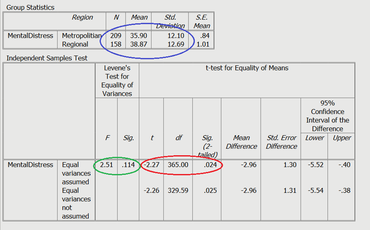
Green: Levene’s test
Red: Test statistics
Blue: Means and standard deviations
Green: The first thing you should examine is Levene’s test. If this test is nonsignificant, that means you have homogeneity of variance between the two groups on the dependent or outcome variable. If Levene’s test is significant, this means that the two groups did not show homogeneity of variance on the dependent or outcome variable. In our example, Levene’s test is nonsignificant so we can move on to the statistics for the tests under the condition of equal variances assumed.
You should notice that there are two lines or rows of statistics given in the output. The first row, which we are using, provides statistics for the tests under the condition of equal variances assumed. The second row, which we are not using, provides statistics for the tests under the condition of equal variances not assumed.
Red: The next thing you should look at is the t value, the degrees of freedom, and the p value statistics in the first or top row of the output. The p-value of .024 shows that there is a significant difference in levels of mental distress reported by metropolitan and regional Australians. If we look at the mean scores, we can tell that regional Australians reported higher levels of mental distress (38.867) than the Australians who live in major cities (35.904).
You will also notice that there is a 95% CI presented, which is a 95% Confidence Interval of the difference. This CI has a lower limit at -5.525 and an upper limit at -.401. Because the CI does not include 0 we can infer that the difference between the two groups does exist in the population.
Blue: Next, make sure you have a look at the mean, standard deviation, and sample size (N) for both groups. You can get the effect size (Cohen’s D) by using an effect size calculator.
You may find an effect size calculator here: https://www.socscistatistics.com/effectsize/default3.aspx
If you enter the mean, standard deviation, and sample size for both groups, you should get a Cohen’s D of .239.
Independent T-test Write-Up
You will need to report the Means and SD for each group, along with the t test statistic (t), its p value, and its effect size d.
It is common in many formats to round your decimal places to two. Therefore, a Write-Up for an Independent T-test should look like this:
An independent samples t-test showed that the metropolitan sample (M = 35.90, SD = 12.10) reported lower levels of mental distress (t=-2.27, p=.024, d=.24) than the regional sample (M = 38.87, SD = 12.69).
