6.3 GNSS Accuracy
There are different levels of accuracy of GNSS measurements, and these are directly related to the technique and equipment used, as well as the length of the observation times.
SP1
In Australia, the way we describe and determine accuracy is outlined in the Intergovernmental Committee for Surveying and Mapping (ICSM) Special Publication 1 document, which is referred to as SP1. ICSM is a group made up of surveyors and other spatial science professionals from each of the State and Territory Governments, along with representatives from Geoscience Australia.
SP1 is the document that sets out the standards for survey control (permanent survey marks) in Australia, and has six guidelines that cover the different methods of surveying that can be used to generate coordinates for permanent survey marks. These guidelines provide information on the methods and techniques needed to achieve different levels of accuracy, which is defined by the principle of uncertainty.
Uncertainty
Uncertainty is quite a simple idea – it is the measure of how wrong a value (in the case of GNSS, the coordinates) may be. It is expressed in the same units as the values, so in the case of GNSS it is usually expressed in metres.
For example, if the plane projection coordinates of a permanent mark were 1000m E and 50,000m N, with an uncertainty value of 0.05m in the horizontal that would mean the coordinates of the mark could be wrong by up to 0.05m.
Uncertainty is expressed as a standard deviation, but one that has been expanded to the 95% confidence interval. Remember from Module 0 the area under the curve of the normal distribution is about 68% at one standard deviation from the mean.
What 95% confidence interval actually means is that we are 95% confident that a sample of data will contain the true mean of the population of the data, even though we don’t know what the whole population looks like.
We achieve the expanded confidence interval by multiplying one standard deviation by a coverage factor, which is basically a scaling factor to take one standard deviation (which is about 68%) up to 95%. The coverage factor is represented by k.
The formula for uncertainty is:
95% CI = 1 x k
x k
Where 95% CI = 95% Confidence Interval
= standard deviation of sample
1.996 = coverage factor for one dimension
Uncertainty in two dimensions
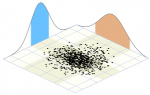
For horizontal coordinates, we have two dimensions, so we can describe uncertainty as an ellipse, where one axis is representing the uncertainty of one horizontal direction (such as Easting), and the other ellipse axis represents the other horizontal direction (such as Northing).
Because we are dealing with data in two dimensions, and each has its own standard deviations, we have two normal distribution graphs that combine to mean the area under them is three dimensional. The easiest way to visualise this is to imagine two normal distribution curves are placed at a right angle to each other, their x axes are now the axes of the ellipse, like in figure 6.3(a). This is known as a Gaussian bivariate normal distribution. When there are more than two dependent variables, it is known as a multivariate normal distribution.
At one standard deviation, the area under these two normal curves is about 39%, so a larger coverage factor is needed. Thus, the equation for uncertainty for two dimensions is:
95% CI = 1 x 2.448.
Where 95% CI = 95% Confidence Interval
= standard deviation of sample
2.448 = coverage factor for two dimensions
Uncertainty for three dimensions
To describe the uncertainty of a combine horizontal and vertical coordinate, we need a three-dimensional shape. Enter our old friend the ellipsoid!
To deal with the third dimension, the third normal distribution can be added to the two dimensional normal distributions, much like the axes for a Cartesian coordinate system. The area under the three curves at one standard deviation is about 20%, so the coverage factor is 2.796 to expand to the 95% confidence interval. From above, this is known as a multivariate normal distribution.
The equation for uncertainty in three dimensions is:
95% CI = 1 x 2.796.
Where 95% CI = 95% Confidence Interval
= standard deviation of sample
2.796 = coverage factor for three dimensions
Types of uncertainty
Regarding survey data (including GNSS data), there are three main types of uncertainty. Survey, relative and positional. Each is used to describe a particular type of uncertainty that is useful in surveying, and all are expressed at the 95% confidence interval.
Survey uncertainty is the uncertainty of the coordinates (vertical and/or horizontal) of a permanent survey mark within a survey, without considering any uncertainty of the coordinates of the datum realisation. This means that we are looking at the uncertainty of the survey independent of the datum.
Relative uncertainty is the uncertainty of the coordinates (horizontal and/or vertical) between any two permanent survey marks. They would usual be from different surveys.
Relative uncertainty is useful in understanding the accuracy of different types of surveys, potentially using different techniques, by comparing their uncertainty values.
Sometimes relative uncertainty may be expressed as a ratio.
Positional uncertainty is the uncertainty of the coordinates (horizontal and/or vertical) of a permanent survey mark when its coordinates are considered with respect to the datum. This is basically the final level of uncertainty that a permanent mark can get, it indicates it has been included in some kind of large survey network adjustment. It is the uncertainty value that is recorded any of the government survey control databases.
Survey uncertainty for GNSS
Now that we have a framework to discuss accuracy of GNSS data, we can examine the survey uncertainty of each type of GNSS observation techniques we have learnt about in Chapters 4 to 6.
Figure 6.3(b) is taken from the Guideline for Control Surveys by GNSS – SP1 Version 2.1, and it outlines the survey uncertainty of all the code and phase observable techniques we have discussed.
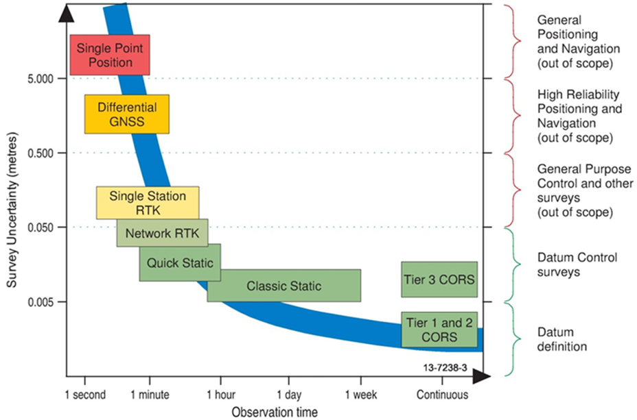
As SP1 is dealing with survey control, the code observable techniques are noted as out of scope. This means they are not discussed in SP1 as they are unable to achieve sufficient accuracies to contribute to assigning coordinates to permanent survey marks to be included in control surveys.
