In point positioning, we use the code part of the signal to determine the satellite range, however, for a series of reasons we’ll discuss soon, this range isn’t actually the correct range, so we refer to it as a code pseudo range.

Code pseudo range positioning works on the simple idea that each GNSS receiver has a copy of the codes each satellite transmits (remember that each satellite, apart from GLONASS, have unique codes) and that the receiver can compare the code it receives with the code it has on board to determine the difference between them. This is shown in Figure 4.3(a).

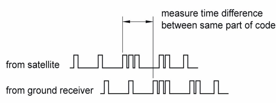
The receiver identifies the code it should be hearing from a particular SV at a particular time, and compares it to what it has received. The difference between the two codes is the time delay, which can then be used to calculate the distance to the SV.

This assumes that the signal generated by the GNSS receiver is produced at exactly the same time as the satellite generates and sends the signal, however, GNSS receivers only have quartz clocks, which are nowhere near as accurate as the atomic clocks that SVs have.

Now we have two problems to solve, the signal delay and clock differences. BUT using the fourth satellite can help us resolve this! BUT…satellite orbits and atmospheric errors also impact our signal!

This is why code pseudo ranging has five fundamental components.

Step 1: Trilateration

The fundamental concept that allows us to generate a position in point positioning is the technique of trilateration, as discussed in section 4.2 – we can determine our position using three satellites ranges.

Step 2: Satellite code pseudo ranging

The satellite and receiver should be generating the same code at the same time, and by understanding the delay in the satellite code in getting to the receiver, we can determine the distance/range to the satellite. This can be shown by the equation:

However, as we’ve already recognised, there can be issues accurately determining ranges due to clock errors.

Step 3: Four satellites for X, Y, Z & time

The issues with accuracy and time of the clocks in SVs and GNSS receivers is referred to as clock error or clock bias, and both satellites and receivers are subject to these errors. Clock errors impact the ability to accurately measure the range, as the time a signal takes to reach a receiver cannot be accurately determined.

Before GNSS chips started appearing in smartphones and devices connected through telecommunications networks, the quartz clocks in GNSS receivers had no central system to align themselves to. This meant they needed an external source to confirm their time, much like when a watch has a new battery put in it – it can tell time, but until it is set relative to a time zone, it isn’t particularly useful. This meant that GNSS receivers relied on receiving satellite signals to adjust their clocks. Now that most devices capable of point positioning are connected to telecommunications networks, their capacity to be aligned to time systems is much more sophisticated, which results in a lower level of clock error, but does not remove it completely.

The way we are able to resolve the clock errors in point positioning is by using the fourth satellite measurement we discussed earlier.

Modelling clock errors

Note: The equations included in this section are not required to be memorised, but are included to assist in explaining the process of removing clock errors in code pseudo ranging.

For this next section, let’s assume we’re using GPS time.

The first clock error is the difference between the satellite clock reading and GPS time at the moment of signal emission, and the second is the difference between the receiver clock reading and GPS time at the moment of signal reception.

We can determine the first by knowing the time the satellite clock reads when the signal is sent, the delay of the clock relative to GPS time, to give us the true time that a signal is sent. In equation format, this looks like:

We can now determine the second clock error by knowing the reading of the receiver clock when it receives the signal, the delay of the clock relative to GPS time, to give us the true time that a signal is received. In equation format, this looks like:

From our previous time delay equation, we already know that the time delay is equal to the difference between the time the satellite emits the signal to when it is received, so we can substitute in our clock error equations:

To determine range, we now have the equation:

The atomic clocks on SVs are monitored by the control segment, and are kept aligned to a specific time, so the corrections for the SV clock offsets  can be assumed to be compensated for (there is some residual offset, but for the purposes of this course we can assume it is zero).

This now means that when a receiver is first turned on, the time difference between the receiver generated code and the received code from the satellite will have two components, the measure signal travel time t(GPS)) and the receiver clock error (_u). This now means our previous range equation can be once again reorganised: R = ct(GPS) –_u).

This range equation can now be used to determine the position of our receiver, and solve the clock bias.

Determining position using pseudo ranges

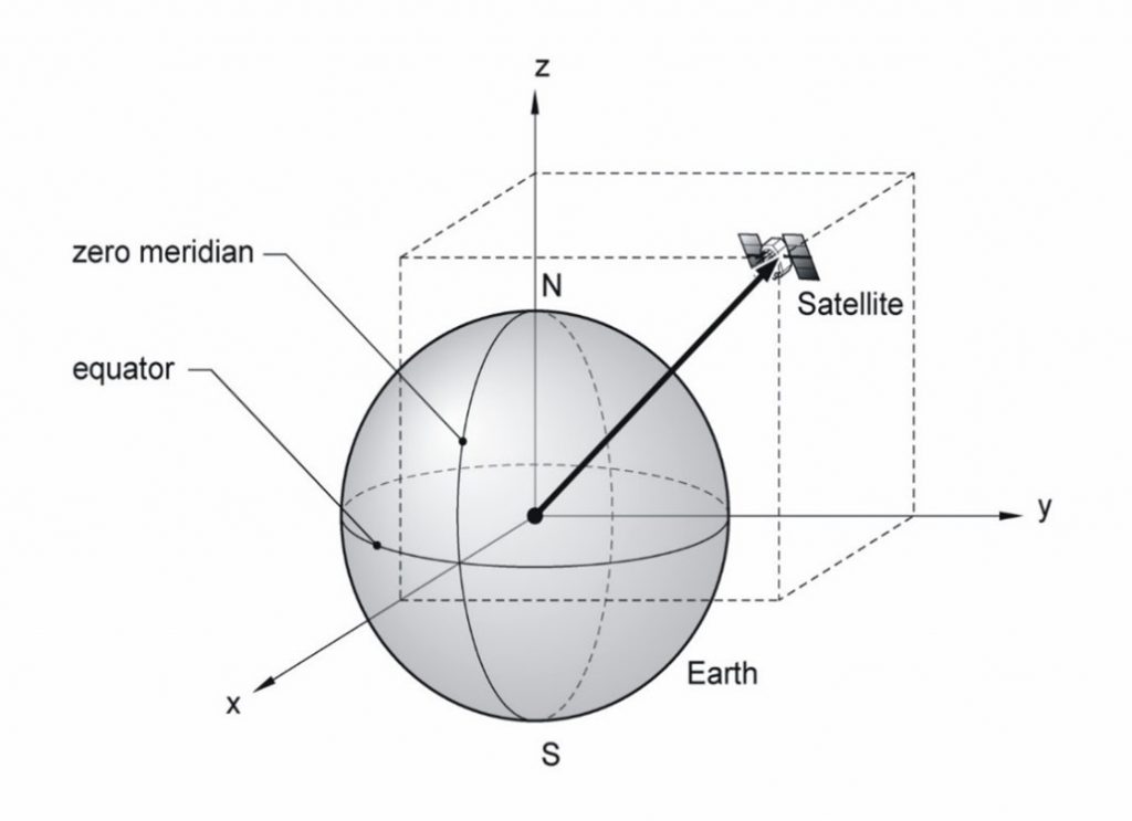
As covered in previous modules, the position of satellites is described in an ECEF Cartesian coordinate system, as shown in Figure 4.3(b).

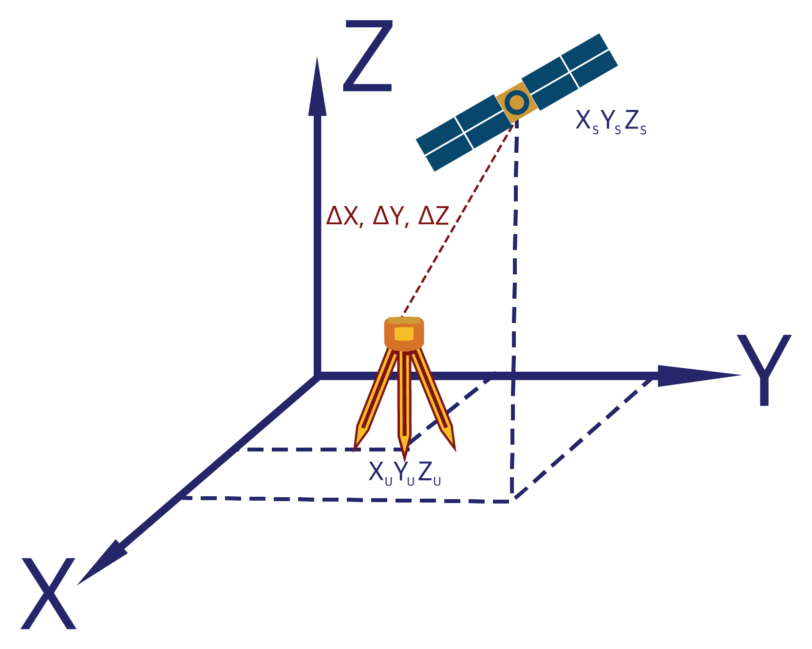
The range from a GNSS receiver to a satellite, as shown in Figure 4.3(c), can be given by the equation:

Where R = Range from receiver to satellite

= difference in the X axis of satellite and receiver

= difference in the Y axis of satellite and receiver

= difference in the Z axis of satellite and receiver

Taking the clock error from the previous section into account, the equation can be given as:

_u

We now have four unknowns in our equation; the position of the receiver in three axes, and the clock error.

Each satellite range will have its own equation, and we know we are able to solve the receiver position with three satellites (three range equations with three variables), so with four satellites we are able to solve for the clock bias as well.

Step 4: Orbit errors

But the satellites are moving! And so are we!

In simplistic terms, we account for the fact satellites and the receiver are moving by:

• assuming the position of the satellite from the code pseudo range values and the ephemeris data
• use the time delay to rotate the Earth the amount it would have moved in that time, and recalculate the position of the receiver
• range is then recalculated between the new receiver position and the estimated satellite position, to give a new estimate of time delay.

The process continues until the range or the time stop changing (this is called ‘converging’ in a maths context), giving a new range value, and thus a more accurate satellite position.

Step 5: Atmospheric corrections

As discussed in the errors section of Chapter 3, the ionosphere and troposphere delay GNSS signals by causing them to refract due to charged particles and water vapour respectively.

In code pseudo range positioning, the GNSS receiver will make estimated corrections for these delays, and apply them when calculating position.

Code pseudo range positioning summary

As you have seen throughout the discussion of code pseudo ranging, the range measured is adjusted and corrected for a variety of factors, but can still not be considered the true range from satellite to receiver, hence the reason it is called pseudo range.

Point positioning using the technique of code pseudo ranging utilises the code observable from four satellites to determine a 3D position by applying a series of mathematical processes:

1. trilateration
2. satellite code pseudo ranges
3. utilising four satellites to solve four unknowns
4. orbit error correction
5. atmospheric error correction