6.2 Baselines
Baselines
We’ve discussed baselines previously – they are essentially a vector that represents the difference in position of two points.
Imagine you have two GNSS receivers that are capable of reading the phase observable, one is on mark 1 and one is one mark 2. You could get an autonomous position on them using code pseudo ranging or DGPS, but we know these are subject to significant errors. Getting a more accurate position means we need to use the phase observable to create a baseline between the two marks. But for now, let’s assume that we have collected the positions of the two marks.
The two receivers are shown in Figure 6.2(a), in a Cartesian coordinate system, and they each have a known position. To calculate the baseline, it’s a simple case of calculating the hypotenuse of two right angled triangles.
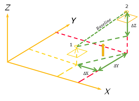
The first hypotenuse (or distance) we need to calculate is the horizontal distance between marks 1 and 2, which is simple given we can quickly determine our  and
and  values by subtracting the position of mark 1 from the position of mark 2. We can then use Pythagoras’ Theorem to solve for the hypotenuse:
c2 = a2 + b2
Where c = Hypotenuse
a =
b =
Substituting into Pythagoras’ Theorem this gives:


We can now project or push this hypotenuse up to the level of mark 1, and by using the value – the difference between the heights of the marks in this case, we can make another right angle triangle. This time we have:


Thus, our baseline between mark 1 and mark 2 can be described by the equation:

But because we are attempting to measure the positions of the marks more accurately than the code observable can provide, we need another way to determine the baseline without starting positions of the marks.
Imagine if we knew a way to determine the distance between two objects using the actual GNSS signals? Oh wait….
The phase observable
Note: If you need a refresher on signals, head back to Chapter 3 as we won’t be discussing all the basics again here.
The phase observable section of GNSS signals is the carrier wave – the blank wave that is modulated with the binary code to become the modulated carrier wave. The code is unique to each satellite in most systems (remember that GLONASS is the exception).
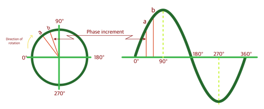
The carrier wave is a 3D wave, and is a right hand polarised wave. This means if we were able to look down the centre of the wave in the direction it was travelling, it would appear to rotate in a clockwise direction, as shown in Figure 6.2(b).
When the carrier wave gets to the GNSS receiver, the first measurement that it observes is a partial wave, which is also referred to as a partial phase, and is represented by or by upper case Greek letter delta (used to indicate change or difference) and lower case Greek letter Lambda (wavelength)  .
.
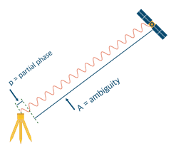
The GNSS receiver is in theory able to measure this partial phase quite accurately – to around of the wavelength. This equates to around 2mm for GPS L1 or L2 signals.
The remainder of the signal is a number of full wavelengths, but unlike code, it’s pretty difficult to know exactly how many of the full wavelengths there actually are as they all look the same, and there’s no distinct start or end. This unknown number of full wavelengths has to be a whole number (as the GNSS receiver already read the partial phase) and is known as the ambiguity, represented by , as shown in Figure 6.2(c).
Combining the ambiguity and partial phase, we now have a range equation for phase observable:
R = ( p + A)
Where R = range
p = partial phase
A = ambiguity
= wavelength
Solving for A is the critical component in GNSS surveying.
So how do we go about this?
In theory the carrier wave wavelength for each signal is a known value, and travels at the speed of light, so the range between the satellite and the receiver could be calculated easily, however, we know that there are a number of errors that impact this calculation.
Imagine if we knew a way to determine the relative distance between two objects another way? Oh wait…
Now we have an equation for range that uses the baseline approach, as well as the signal information:

Differencing
As you’ve no doubt started to realise, most of GNSS positioning involves having more than one of something – satellites, receivers, epochs – to remove errors and solve unknowns from a single thing – satellite, receiver, epoch – and phase observable techniques are no different in solving for ambiguity. With the added bonus of removing a whole lot of errors.
In phase observable we refer to this technique as differencing – the process of using the difference between two things to create baselines. We’re not going to cover the maths behind this in this subject, however, it is important to recognise that each type of differencing has its own equation to describe the baseline (remember back to the range equations in DGPS for a rough indication of how these look). The combinations of these equations help us solve the final baseline equation by getting rid of different variables.
There are three main types of differencing.
Single differencing
Single differencing can happen between two receivers and a satellite, or two satellites and a receiver. Essentially, it’s two observations that are assumed to be happening at the same epoch. Let’s look at the two receiver scenario first.
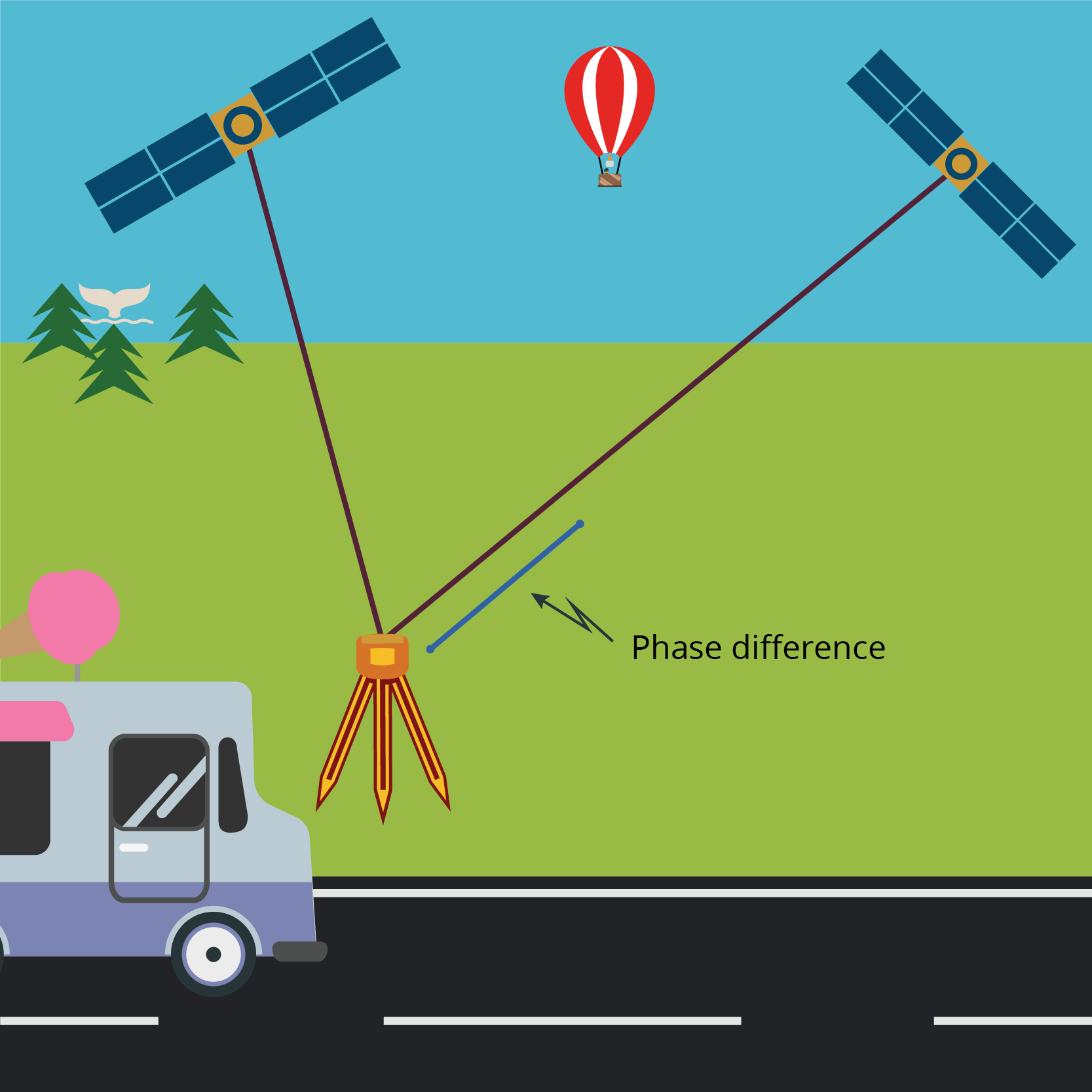
As shown in Figure 6.2(d), a common satellite is broadcasting a signal that is being received by two receivers. If we assume we know the partial phase at each receiver, and assume the range from the satellite to the receiver on the left is fixed, we can remove this range from the longer range of the receiver on the right, leaving us with a phase difference. As you should remember from the DGPS module, this combination of satellite and receivers means we can remove the satellite clock error from the range as well
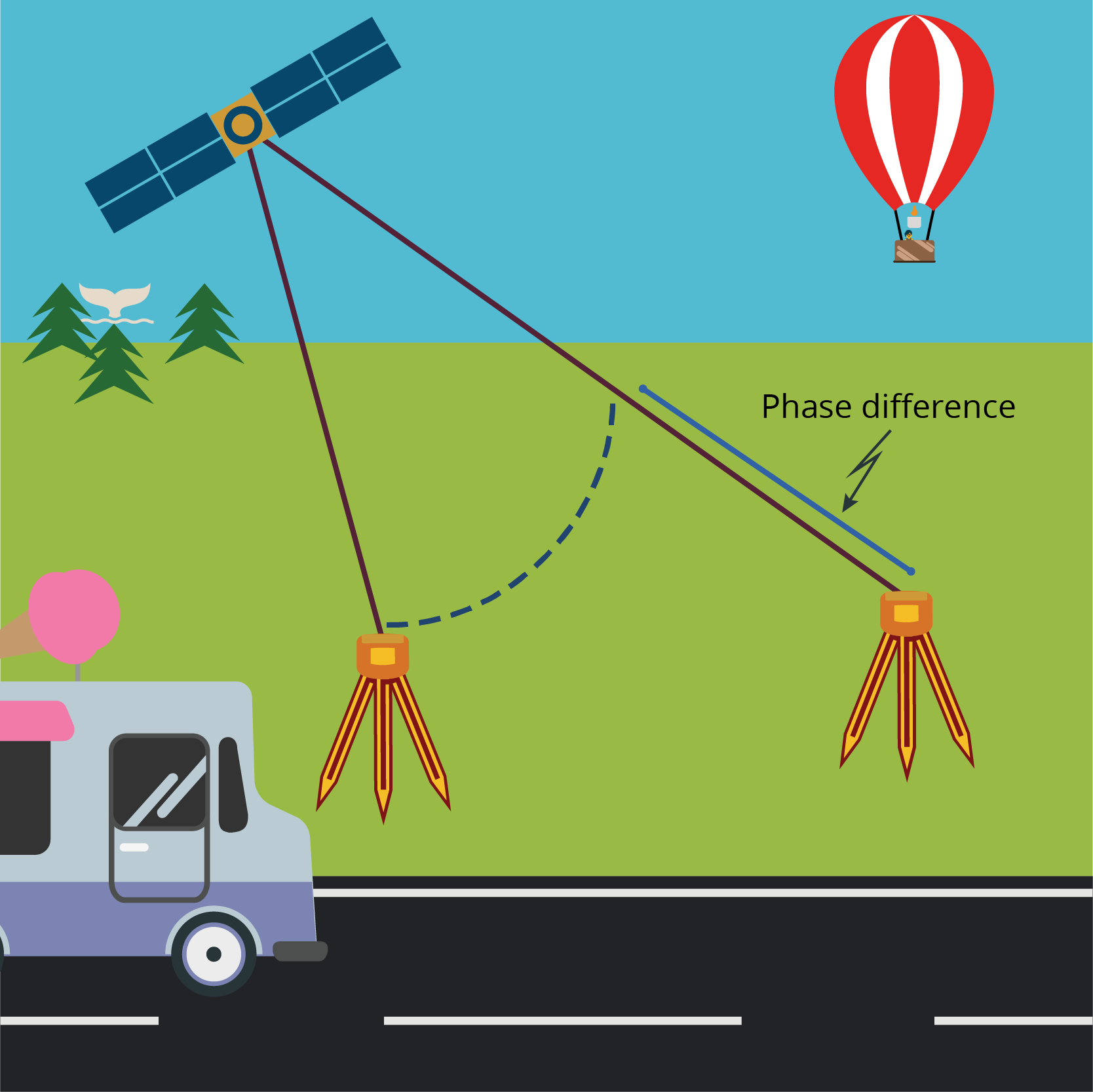
Depending on the locations of the receivers, this method of single differencing may also have a significant impact in reducing the atmospheric errors if the receivers are relatively close. The signal is passing through similar atmospheric conditions so the error is considered to be similar for both measurements, and thus can be considered resolved or cancelled out.
Orbit errors are also reduced in this method of single differencing, for the same reasons as the atmospheric errors.
The next type of single differencing is when we have two satellites and one receiver, as shown in Figure 6.2(e). As with the one satellite, two receiver single differencing, we can determine the phase difference, but this version removes the receiver clock error.
Double differencing
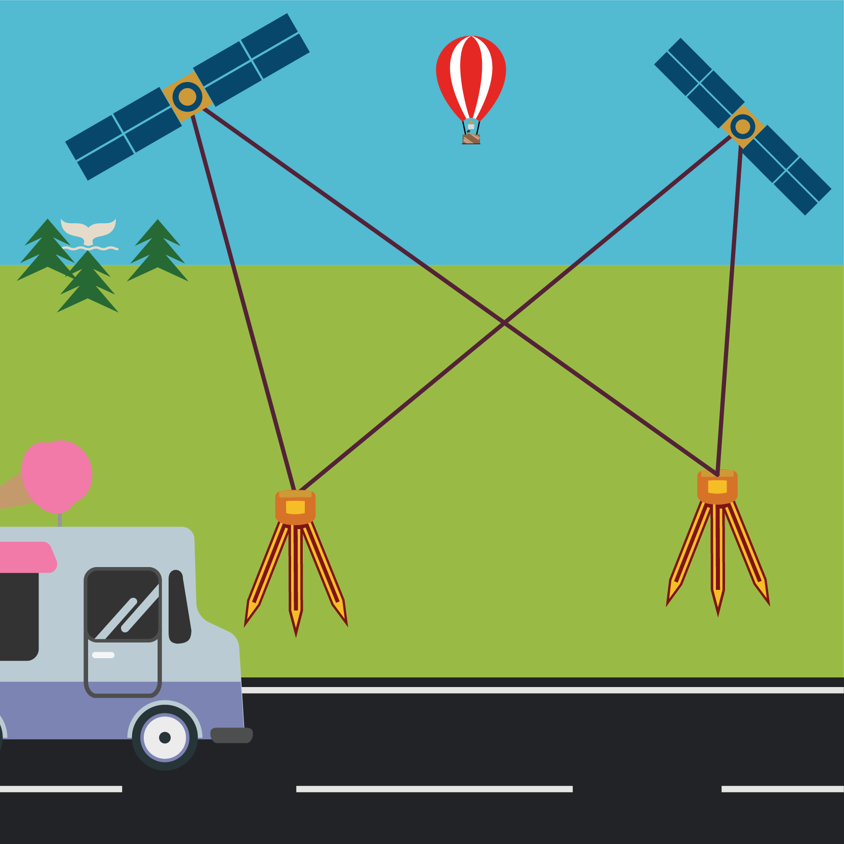
When we combine these two versions of single differencing, we get double differencing, as shown in Figure 6.2(f). Double differencing is four observations, which are again assumed to be happening at the same epoch. We now have sufficient measurements that the satellite and clock errors are dealt with, and the phase differences can be used to determine a baseline between the two receivers, but only if we can solve the ambiguity.
Triple differencing
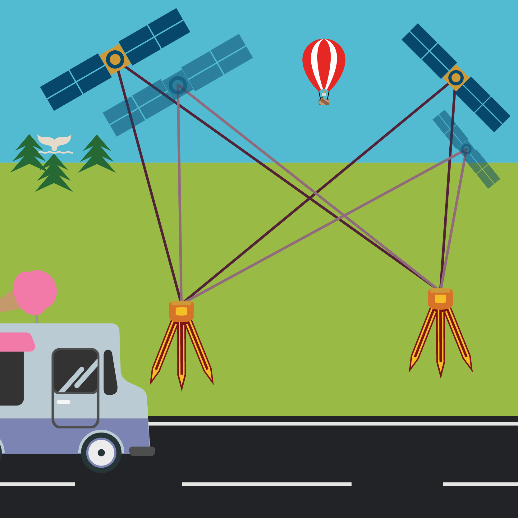
All that we really have left to help solve for ambiguity is epochs, so if we took two lots of double differencing, at two different epochs, you guessed it, triple differencing! This is shown in Figure 6.2(g).
While we’re not going to get into the maths of it in this subject, the triple differencing maths is quite beautiful, as all of the ambiguities of the different signals cancel each other out. This leaves us with an equation for the baseline between the receivers that can be used to provide an estimated value of the baseline.
Solving ambiguity
The baseline equation in double differencing isn’t solved by triple differencing, but the estimated baseline value can be put into the double differencing baseline equation. This allows the receiver to re-estimate the ambiguities as it now has a rough baseline. This refined ambiguity value then can be used to improve the baseline estimate, and so on. This is the mathematical process of iteration.
While these iterations are occurring, the receiver is tracking more satellites to be able to solve the double differencing baseline equation. This equation has four unknowns; the three position unknowns – ( ) as well as the ambiguity value A. To solve for four unknowns the receiver needs four independent observations – four sets of double differencing. This means we need five satellites to solve the baseline.
This process of resolving the ambiguity using double differencing happens in two stages:
- An initial estimate of the ambiguity is made using the triple differencing baseline estimate. This estimate is a number with a decimal place, which in computer science or programming language is called a float value or float data type. Using this estimate, a baseline solution can be estimated, but because it’s not very accurate, it is referred to as a float solution.
- Once the float solution has been determined, and the receiver and software has measured enough independent double differenced solutions, it turns the float value solution of into an integer value, which is a whole number. At this point the ambiguities are considered to be resolved, and the receiver can provided a fixed solution as it has solved the unknowns.
A fixed solution is about 10 times better than a float solution in terms of accuracy. Given the number of satellites in orbit from different GNSS, a fixed solution should be the preferred option when undertaking phase observable techniques, particularly for those techniques that utilise a GNSS rover for undertaking measurements.
In summary
- Single differencing is two observations at the same epoch,
- two receivers and a satellite eliminates the satellite clock errors, and significantly reduces the atmospheric and satellite orbit errors
- two satellites and a receiver eliminates the receiver clock errors.
- Double differencing is a combination of the two single differencing methods, and removes satellite and receiver clock errors, as well as reducing the orbit and atmospheric errors as mentioned in single differencing.
- Triple differencing is two sets of double differencing with the same receivers and satellites, but at different epochs. It eliminates the ambiguity term and allows for the baseline equation to be solved once 4 independent double differenced solutions are observed.
- A float solution is when the ambiguity value is estimated as a float value i.e. with a decimal place.
- A fixed solution is when the ambiguity is resolved as an integer value – a whole number.
Carrier phase errors
While it outside the scope of this course, it is important to note that an error know as cycle slip can occur in phase observable techniques. This is when the signal is lost temporarily and the counting of the number of full cycles needs to commence again. This causes a jump in the data, as the integer changes. This is covered in the Geodetic Surveying A and B courses in more detail.
Baselines + Coordinates
The phase observable measurement technique in GNSS has allowed surveyors to measure to levels of accuracy that were previously unachievable without decades of measurement.
By applying coordinates to relatively accurate networks of GNSS baselines, the state and national survey control networks – those networks of permanent survey marks that have accurate coordinates on them, have significantly improved in a relatively short timeframe.
The combination of this level of accuracy, and the significant distances that baselines can be generated over has meant surveyors have an additional suite of tools and techniques at their disposal to complete their work. Not only has GNSS surveying made certain activities faster, but also significantly safer in some application areas, as drones have in recent years for engineering and mining. The next section will discuss how accuracy is measured in GNSS surveying, followed by a summary of the different techniques used in GNSS surveying.
